|
Nesbit or Kwon or MacKenzie?
Dave Tutelman
-- Dec 6, 2018
Appendix
This appendix covers some of the more technical points in the analysis on the second page.
If you're not into math, you don't need to read this
(and probably won't get much from it). I go into some of the equations
here, but there is no attempt to be completely rigorous. This would
never be accepted as a degree thesis by a graduate school. That doesn't
mean it's wrong, just not a complete analysis. The point here is to
give some idea of the math and the engineering knowledge that led me to
my assertions on the second page.
When I was in engineering school around 1960, there wasn't as much
specialization as today. My degree was in Electrical Engineering, but I
had to take courses in Mechanical and Civil Engineering as well. I
learned that there were direct analogues of electrical systems in both
ME and CE. By
"direct analogues", I mean that the mathematical equations are the
same,
and you can even identify the quantities that represent one another in
the different disciplines. On several occasions, I used those analogues
to analyze something about mechanics or materials that surprised my
professors; ME or CE students would not have gotten to those particular
analysis
tools before senior year or even graduate school. (In fairness, there
were relatively few components that electrical engineers had to learn
about, compared with mechanical engineers. And circuits using those few
components required
frequency and transient analysis. So EEs had both
the opportunity and the need to learn the techniques early in
their education.)
So
I do have engineering experience and intuition in the technical details
here. That said, let's look a little more deeply into analysis of the
shaft bend during the downswing.
The basic bending equation
The most elementary, fundamental formula for flexural bending goes back
over 250 years. About 1750, Euler and Bernoulli
(names ranking just
below Newton in pantheon of physics and math) proposed an equation for
the flexural bending of
a beam. It is still the  basic
equation at the beginning of the chapter on bending in any engineering
text. basic
equation at the beginning of the chapter on bending in any engineering
text.
where:
- R
is the radius of curvature of the beam at some point x
along the beam. (See the diagram to the right.) By the way, a golf
shaft is a tubular beam of varying diameter. It is definitely governed
by the
Euler-Bernoulli equation.
- M
is the bending moment at point x
along the beam. Most of the art of using Euler-Bernoulli is figuring
out M(x) at each point on
the beam.
- E
is the elastic modulus of the material at point x.
(Always positive.)
- I
is the area moment of inertia of the cross-section of the beam at point
x.
(Always positive.)
- You can't measure E
nor I
easily for a golf shaft. But it is possible to measure the shaft's
stiffness
non-destructively, which is E
times I.
Fortunately, all the bending equations have the
product EI
rather than either one separately. Almost all engineering situations
dealing with shaft bending deal with EI
as a single quantity that varies with x.
(An exception to this rule is the design itself of the shaft. The shaft
designer has to
choose materials, orient them for strength where he wants it, and deal
with diameters and wall thicknesses. That engineer deals with E
and I
separately to accomplish the EI(x)
that will govern the shaft's performance.)
- The inverse of the radius of curvature is the
curvature itself. So the left side of the equation is the curvature of
the shaft,
the sharpness of the bend, at point x.
In engineering texts, where you are assumed to know calculus and
the mathematical meaning of curvature, the Euler-Bernoulli equation is
usually written as:
In calculus, the second derivative of a nearly horizontal
curve is its curvature. Expressing it this way enables its solution as
a second order differential equation. Also -- important to this
specific debate -- it explicitly controls the sign (the direction) of
both moment and curvature.
Before we leave this simple equation, let's do some simple algebra and
solve for M.
Let's call this the "moment
form" of the Euler-Bernoulli
equation. We will be using the equation later, so it is convenient to
have a name
for it.
 Bending needn't be
any
more complicated than this equation. If you know the
curvature at point x,
then you know the bending moment at point x.
You certainly know the direction of the bending moment, which is what
this debate is about. Bending needn't be
any
more complicated than this equation. If you know the
curvature at point x,
then you know the bending moment at point x.
You certainly know the direction of the bending moment, which is what
this debate is about.
So
what do we know about the direction of curvature near the handle? In
the 1990s, TrueTemper built an instrument called ShaftLab. It was data
capture of shaft bend during the swing, and the bend was measured
directly by
strain gauges attached to the shaft just below the grip of the club.
Maybe not precisely at
the hands, but quite close -- definitely close enough.
And
what did ShaftLab show? At impact, the shaft is always bent forward
where the strain gauges are.
The Euler-Bernoulli equation says that means the bending moment
(torque) applied to the shaft by the hands is negative at impact.
But this is
static. Steady state. We want to know about a shaft while it is being
swung.
Yes, there are some differences, some additions. But you ought to note
that the Euler-Bernoulli equation still rules, though there may be some
dynamic forces as well as static ones producing the bending moment. The
main examples are:
- If an adjacent segment of the shaft (at z-Δz)
is
deflected, that will produce a bending tug on the adjacent segment at z.
- The bending of the shaft produces friction. The
friction force is in a direction opposite to the motion producing it,
and is proportional to the rate of bending; faster bending means more
friction.
Let's look at the equations of motion for dynamic bending.
|
Equations of
motion
The
homogeneous equation
The model of the shaft is a second-order differential equation. It is
solved as a homogeneous
equation (that is, the free-body response with no external
forces or torques applied) and a set of boundary conditions
representing those external influences. Let's start with the
homogeneous equation, equation (2) in the paper.
 The first thing to notice is that the equation tells
us the three dimensions of the analysis: The first thing to notice is that the equation tells
us the three dimensions of the analysis:
- The t
dimension, of course, is time.
- The z
dimension is the axial
distance, the measurement along the shaft's axis.
- The y
dimension is the deflection
in the swing plane. This is a 2D analysis, where the plane of interest
is the swing plane. (The "alpha" direction.) There was no attempt to
model cross-plane deflection (called "droop" or "beta deflection") nor
rotation around the shaft
axis ("gamma"). Of course y
changes with time. It also changes with z;
the deflection is different as you move along the shaft.
The next thing to look at is what the three terms of the equation
represent.
- In the first (blue)
term, mz
is the mass per unit length, and the second partial derivative is the
acceleration of the deflection. So it is F=ma
for each increment of shaft length. What it says is the propagation of
deflection along the shaft is determined by the mass per unit length.
If the mass of the shaft itself were zero, the term would not be there
and there would be no wave propagating along the shaft. Put another
way, the mass of the shaft is the only thing preventing the entire
shaft to bend like an ideal spring. The shape would be similar at all
times, with only the amplitude being different.
- In the second (yellow)
term, c
is a damping or friction factor, and the partial derivative is the
velocity of the deflection. This accounts for damping of the shaft's
vibrations, specifically the damping due to the shaft's internal
friction. The damping term
is acting as a dashpot (if you're mechanically inclined) or a resistor
(if you're electrically inclined) where it sits in the equation.
- The third (red)
term looks a little like the Euler-Bernoulli equation. Look at the part
inside the square brackets. It is what we earlier named the "moment
form" of the Euler-Bernoulli equation. Note that EI
is correctly identified as a function of z;
that is, EI
varies along the length of the shaft. The butt of any golf shaft will
be stiffer than the tip, and that variation is mathematically expressed
as EI(z).
The variation of EI
shown in Figure 7 of the Nesbit-McGinnis paper is very reasonable for a
shaft, rather
middle-of-the-road. So that can't be the difference between Nesbit's
model and well-known shaft behavior.
The terms of the homogeneous differential equation say mathematically
that the wave
motion along the shaft and the
damping of the shaft have
to balance out the moment
necessary to create a bend in the shaft.
|
Initial
and boundary conditions
- The homogeneous equation is the behavior of the
system after it has been tweaked or plucked, as it settles back to
steady state.
- The initial conditions specify exactly the state at
some point in time (t=0
in this analysis, and in most analyses).
- The boundary conditions are where the external
drivers
(forces and torques, in a mechanical problem like this) are added to
the system.
Let's look at how Nesbit and McGinnis set up the initial and boundary
conditions, based on this view of the shaft.
The z-axis
runs from zero at the hands to L
at the tip. All the external forces and torques are applied by the
clubhead to the tip of the shaft. Here are the equations for the
boundary conditions.
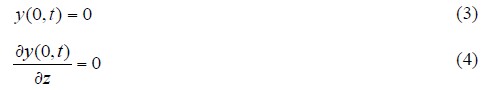
Equations (3) and (4) are the boundary conditions at z=0
for the entire time of the simulation. The equations constitute the
enforcement of the cantilever
assumption.
They say that at z=0,
where the shaft is under the hands, the position (y)
is zero and the slope (y')
is zero -- meaning the shaft comes out of the hands with no slope,
perfectly flat. These equations completely determines the
influence of the hands on the shaft, and setting them to zero assures
that the hands will behave as a clamp. There will be no damping at the
hands at all. From
our damping experiment, we know this is wrong.
If we were going to make the hands a damping grip
instead of a clamped
cantilever, equation (4) would be the place to do it. Instead of
setting the slope to zero, the slope should be on a stiff, lossy,
angular
spring. I haven't worked the problem in detail, and I haven't set up a
problem like this in over 50 years, but my instinct tells
me equation (4) should be something like:
| A |
δy(0,t)
δz |
+ B |
δ2y(0,t)
δz
δt |
= 0 |
In the first term, A
is a spring coefficient for the stiffness of the very stiff pivot
(instead of a perfectly
stiff cantilever). The second term has B
as a damping coefficient which causes more energy loss the faster the
slope changes.
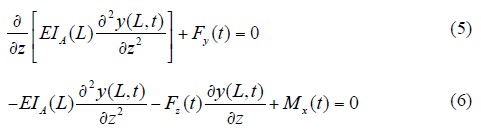
Getting back to Nesbit, equations (5) and (6) are the boundary conditions at z=L
for the entire time of the simulation. The equations are based on the
forces and moments on the tip of the shaft. In the diagram above, those
are Fy,
Fz,
and Mx.
The functions Fy(t),
Fz(t),
and Mx(t) are
prescribed by earlier simulations that determined the forces and
moments applied to the tip of the shaft.
Equation (5) is a balance of forces at the tip of the shaft, those
forces in the y
direction (across the shaft in the alpha plane). Fy
obviously fits this description, but the other term? We recognize the
other term as the derivative (slope) of the moment (it's the moment
form of Euler-Bernoulli) taken along the z
axis. Engineers with experience in beam analysis instantly recognize
the derivative of the bending moment as the shear force (internal
force) across the beam. So the equation says that the imposed y
force at the tip has to balance the internal shear force at the tip.
Equation
(6) is a balance of moments, again at the tip of the shaft. The third
term is obviously a moment; it's the externally imposed moment at the
tip. The first term we should by now recognize as the moment form of
Euler-Bernoulli, so it is a moment. That leaves the second term to be
interpreted as a moment. Let's look at that. Fz(t)
is the component of force F(t)
along the z axis. With a straight shaft, that would be pure axial force
on the shaft, trying to stretch it rather than bend it. But we are
dealing with a deflected shaft; the derivative in the second term is
the slope of the shaft at the tip. So Fz(t)
resolved itself into an axial component (trying to stretch the shaft)
and a radial component (trying to bend back towards straight). If we
multiply Fz(t) by
the slope, we get the radial (bending) component. Well, there's this
little confusion between the tangent and the sine; but for small enough
angles they are close to the same (and the tip is bent maybe 2-3
degrees, which is small enough).
For the record, I just gave a
hand-waving justification, not a rigorous one. I'm unhappy with it
myself. I just described a term that is a force, not a moment. I am
unable to find a moment arm, a distance, to go with the bending force I
described. Having drawn a few diagrams, I think I would be happier if
the term were:
- Fz(t)
y(L,t)
That would at least be a bending moment in a direction to reduce the
bend, and would also be consistent with the diagrams I drew.
Rather than boundary conditions, equations (7) and (8) are initial
conditions. They apply at t=0,
and they apply for all z
-- that is at every point on the shaft.
Equation (7) says the shaft is straight at the beginning of the
downswing, which is
just plain silly.
During the transition (the start of the downswing), the shaft is bent
anywhere from 40% to 100% of the maximum it will bend during the
downswing.
Where it lies in this range depends on the way the golfer loads the
shaft, but I have never heard of a swing with anything vaguely
resembling a straight shaft at transition. Try it yourself. Find any
good golfer's driver swing on YouTube, face-on slow-motion. Freeze it
at the exact moment of transition and lay a straight edge along the
shaft as it exits the hands. You'll find the tip substantially in lag
due to bend.
Equation (8) says the shaft is not going into any
bend at the moment of transition. Not only is it not bent, but not
moving towards bending; there is no derivative of y
with respect to time at any point along its length. This also sounds
wrong, but isn't as obviously wrong as equation (7).
In
any event, I'm not making much of a fuss about this error. I doubt that
it has much to do with the question on the table here, which is the
direction of shaft bend and hand couple at impact. I'm sure it warps
other results somewhere, but I'm not going to spend time on it here.
|
An electrical
engineer's view
As I
mentioned above, undergraduate electrical engineers learned certain
analysis
techniques earlier and perhaps more intensively than other engineering
disciplines. Most of those techniques were to deal with transient
behavior of systems, often reactions to step or impulse function inputs
or an alternating input at some frequency or combination of
frequencies. My experience with this sort of analysis on analogues of
mechanical systems gives me a little insight into the elastic shaft
that is the subject of this investigation.
Let's look at two analogues, and see what we can learn from them.
Tuned
circuit
Here's an example of a perfect analogue between mechanical and
electrical systems. It's not a random example
by any means; it relates directly back to oscillation and damping, like
we saw in the damping
experiment.
The two simple systems above, one mechanical and the other electrical,
are direct analogs of one another.
- In the mechanical system, the mass will bounce back
and forth if the dashpot doesn't introduce too much damping.
- In the electrical system, the voltage will oscillate
up and down if the resistor doesn't introduce too much damping.
Looking more closely, here are quantities that are direct analogues in
the two systems:
| Mechanical
system |
Electrical system |
Role in the system |
| Position of mass |
Charge on capacitor |
Main analysis variable x
(or, for electrical, Q) |
| Force |
Voltage |
The "push" in the system |
| Velocity of mass |
Current |
First derivative of x or Q |
| Acceleration of mass |
Derivative of current |
Second derivative of x or Q |
| Spring |
Capacitor |
Proportional to x,
F
= Kx
v
= Q/C |
| Dashpot |
Resistor |
Damping,
energy dissipation,
proportional to x',
F = cx'
v = RQ' |
| Mass |
Inductor |
Proportional to x",
F = mx"
v = LQ" |
Not only that, the equation of motion/charge is exactly the same:
d2x
dt2 |
+ 2cω |
dx
dt |
+ ω2x = 0 |
This is a second-order differential equation where:
- t
= time.
- x
= position or voltage, depending on which system we analyze.
- c
= damping factor. We'll get back to this in a minute.
- ω =
the resonant frequency of the system in radians per second.
If you tug on either system and let go, there will be a transient
response, which may well be oscillation Let's look at the language an
electrical engineer would use to describe
the different types of oscillation.
For
both the mechanical and the electrical oscillatory system, there is a
common description of the behavior. The graph above shows the major
named types of behavior:
- Undamped,
or no damping
- If the damping factor c
is zero, then the oscillation continues forever.
- Underdamped
- If the damping factor c is less than 1, the
response crosses zero at least once. For c
considerably less than 1 (say, less than 0.2 or so), the response
oscillates at an ever-decreasing amplitude. "Underdamped" means it is
damped, but still manages to oscillate somewhat. The red curve has a
damping factor of 0.02, so it gets a lot of oscillation in before it
dies out for all practical purposes.
- Overdamped
- If the damping factor is more than 1, the response never crosses
zero. It really isn't oscillating, just dying out. The blue curve has a
damping factor of 4.
- Critically
damped
- If the damping factor is exactly 1, that is the fastest the system
can "come to rest" for practical purposes. It is also the lowest
damping value where the response never crosses zero. The green curve
has a damping factor of 1.
Now that we have a language, let's see if we can apply it to the damping experiment
we did when we plucked a club with different ways to secure the handle.
We choose a damping factor that makes the curve look like the response
we observed when doing the experiment.
- Clamped
- This is seriously underdamped; the damping factor is .005 and it
loses only about 2.5% of its amplitude each cycle. This matches the
damping I measured in stop-frame on the video.
- Braced
- A damping factor of .2 leaves us about 3 cycles before the amplitude
is too small to notice.
- Hands
- The clubhead passes zero, but then just limps back to zero. Not
critically damped, but certainly not highly underdamped. This graph
uses a damping factor of .5, or half of critical damping.
In
any event, the damping for "clamped" is more than an order of magnitude
lower than either "braced" or "hands". (The ratios are 40 and 100,
respectively.) That says that only 1% to 2.5% of all system damping is
in the shaft. But the equations Nesbit uses for the simulation only
include damping in the shaft.
Transmission
line
The
tuned circuit is doesn't completely explain the behavior of the shaft,
though it gives a strong hint. But it doesn't talk about the flex wave
traveling along the shaft. It only addresses how the shaft mounting or
grip deals
with signals coming up the shaft. So let's look at traveling and
standing waves.
A
good (admittedly not perfect) analogue of the
shaft is an electrical transmission line. This includes the mighty
power lines running across the countryside on tall towers, as
well
as the lowly coaxial or even twin-lead cables that carry a TV signal
around your house. Let's look at the latter.
The
figure shows an equivalent circuit for a transmission line. Yes, it
also has resistance; it is lossy. But that is mostly a factor in power
transmission. TV signals within a home don't suffer much loss, so let's
just look at the inductors (L) and capacitors (C) in the equivalent
circuit. Why restrict ourselves to lossless lines? Because our damping
test showed that the shaft itself (the transmission line) is not where
the losses in the system are happening.
The
equivalent circuit models the transmission line as a
large number of small LC segments. The more and the smaller the
segments, the more accurate the approximation. The actual, perfectly
accurate, model of the transmission line has infinitesimal segments
(approaching zero), and is better described by a continuous
differential equation than the discrete circuit in the diagram.
The L and C obviously
vary from cross-country power transmission to in-home coax cable, and
even coaxial is different from twin-lead. Let's look at some
interesting properties of a transmission line:
- The ratio of
L to C is constant for a particular design of transmission line, no
matter how large or small the approximating segments. If you halve the
length of a segment, you halve both L and C, so the ratio is the same.
That ratio is a characteristic of the line. In particular, the square
root of the ratio [ sqrt(L/C)
] is called the "characteristic impedance" of the cable, and has an
interesting real-world implication we will explore.
- If
I send a signal down a transmission line, it reaches the end and is
reflected back. Or not. The reflection depends on the load.
- If
the load at the end of the transmission line is an open circuit
(infinite ohms), then it is reflected back with no loss of
energy.
- If the load is a short circuit (zero ohms), then it
is also reflected back completely, but with a polarity reversal, + to -.
- If
the load is in between those extremes, part of the energy will be
absorbed in the load, and the rest will be reflected back with or
without reversal; low-ohm loads will reverse the polarity.
- If
you're still with me, it seems obvious that there is some size of the
load that will completely absorb the signal, with no wave reflected
back. That would be the load impedance which is barely too small for
positive reflection and barely too large for negative reflection.
Remember the "characteristic impedance" from the first bullet point?
That is exactly the size of load to absorb all the energy and reflect
nothing back.
- Depending on how much of the wave is
reflected at each end, the transients running up and down the line may
reinforce or cancel one another at different places along the
transmission line and form a "standing wave"
on the line. Standing waves mean that the signal transfer becomes very
sensitive to both the frequency and the exact length of the line.
- But...
with a load at or near the characteristic impedance (also called a
"matched load"), any signal cannot survive much longer than one trip
down the line. A matched load gives a much smoother frequency response.
If the signal is a transient pulse of some sort, rather than a periodic
wave, the signal is received undistorted by the load and never appears
again (because there is no reflection to contend with).
A lot of the properties of a transmission line are shared by our golf
shaft.
- I
don't know of anything about a vibrating beam (or golf shaft)
comparable to a characteristic impedance. Perhaps there is; if not,
perhaps there should be. We will see why below.
- If
the shaft is sufficiently lossless, any signal or wave traverses it at
some characteristic speed until it reaches the end and is reflected
back. Or not. The reflection depends on the load.
- If the
load at the end of the shaft is a rigid clamp, then it is reflected
back with no loss of energy.
- If the load is a frictionless hinge, then it is
also reflected back completely, but with a polarity reversal, + to -.
- If
the load is in between those extremes -- a lossy hinge -- part of the
energy will be
absorbed in the load, and the rest will be reflected back with or
without reversal; low-friction loads will reverse the polarity.
- If
you're still with me, it seems obvious that there is some load that
will completely absorb the signal, with no wave reflected
back. That would be the hinge loss which is barely too small for
positive reflection and barely too large for negative reflection. Let's
call that the "matched load".
- Depending
on how much of the wave is reflected at each end, the
transients running up and down the line may reinforce or cancel one
another at different places along the transmission line. If instead of
transients, we have a sinusoidally varying excitation, it can form a "standing wave"
on the shaft. Standing waves mean that the signal transfer becomes very
sensitive to both the frequency and the exact length of the shaft.
- But...
with a load at or near the matched load, any signal cannot
survive
much longer than one trip up the shaft. A matched load gives a clean
transient response. The
transient signal reaches the load intact and never shows up again.
The
lesson here, guessed from knowledge of how a transmission line works,
is that even if you have no damping in the shaft itself, you can still
have very strong, even perfect, damping if the load at the grip end is
close to the matched load.
|
What's new?
Mike Duffey asked me for a summary of what is new in this December 2018
version, compared with the October version. Here it is.
In the October version, I had a confusing (and probably confused)
argument why higher mode vibrations (harmonics) were not likely
responsible for significant changes of the shape of the shaft, as
Nesbit and previously Brylawski had asserted. In order to clean up my
muddy reasoning, I went into Nesbit and McGinnis' paper on shaft bend.
As a result of that foray, here is my [tighter, I hope] reasoning.
Nesbit and McGinnis report a reverse-bend shape at impact. It is a
lag curvature near the hands that devolves to a lead curvature for the
bottom 40%-60% of the shaft. If true, that would also
explain the positive couple, by simple application of Euler-Bernoulli
bending. But is it true?
Nesbit and McGinnis make several shaky assumptions when they set up the
differential equation for shaft bend. Three of those assumptions
explain the different shaft shape and thus the torque. These assumptions are:
- All damping of the shaft's vibration is in the shaft
itself; none is in the handle and hands. (The paper pays lip service to
damping in the hands, but the equations don't cover it.) Experiment suggests less than 3% of the damping is in the shaft
itself, and more
than 97% is in the hands.
- At impact, the only force or torque bending the shaft is
the eccentric loading due to centrifugal force at the CG of the
clubhead. That assumption is refuted by both empirical data (from
ShaftLab) and analytical modeling (a Sasho MacKenzie paper on shaft
bend).
- The shaft is modeled as a cantilever beam, admittedly for
ease of computation. (Nesbit asserts the shaft/hand interaction is not
sufficiently understood to do otherwise.) This assumption is obviously
questionable, but I don't have a precise refutation beyond its clearly
incorrect implication for damping.
Fixing assumption #1 provides the basis for ignoring higher mode behavior, especially
when you factor in the speed of propagation of a flex wave.. Any
higher-mode wave has no chance to stick around long enough
to affect shaft shape in an important way.
Assumptions #2 and #3 can together explain the reverse bend at impact even
statically. We don't need flex waves, either stranding or traveling, to
create the reported shaft shape. Since #2 is false and #3 is
questionable at best, that negates the whole idea of a
reverse bend in the shaft at impact, a shape also refuted by
ShaftLab measurements.
Last
modified -- Dec 21, 2018
|